06:
We have already discussed the advantage of using shaders to create interesting visual effects. This time we will have to deal with fragment shaders *and* vertex shaders. In a nutshell, a vertex shader takes care of managing the vertices position, color, etc. which are then passed as “fragments” to the fragment shader for rasterization. “OMG, this is so abstract!!”. Yeah, it is less abstract than it seems, but nevertheless it requires some know how. As previously, I really suggest this : I find myself going back and forth to it regularly, always learning new things.
Good, so, what’s the plan? The main idea in the following code is to use a PShape object to encode all the vertices: we basically are making a star shaped thing out of rectangles, which in 3d graphics parlance are referred to as “quads”. Once we have created such a PShape object, we will not have to deal with the position of vertices anymore: all the change in the geometry will be dealt by the GPU! Why is this exciting? It’s because the GPU is much much faster at doing such things than the CPU. This allows in particular for real-time reactive fun. Indeed, the code gets input from the microphone and the webcam, separately. More precisely, each frame coming from the webcam is passed to the shader to be used as a texture for each quad. On the other hand, the microphone audio is monitored, and its amplitude controls the variable t, which in turns control the rotation (in Processing) and more importantly the jittering in the vertex shader. Notice that the fragment shader doesn’t do anything out of the ordinary here, just apply a texture.
Here’s how the code looks like
import processing.video.*;
import processing.sound.*;
Amplitude amp;
AudioIn in;
PImage back;
PShape mesh;
PShader shad;
float t = 0;
float omega = 0;
float rot = 0;
int count = 0;
Capture cam;
void setup() {
size(1000, 1000, P3D);
background(0);
//Set up audio
amp = new Amplitude(this);
in = new AudioIn(this, 0);
in.start();
amp.input(in);
//Set up webcam
String[] cameras = Capture.list();
cam = new Capture(this, cameras[0]);
cam.start();
textureMode(NORMAL);
mesh = createShape();
shad = loadShader("Frag.glsl", "Vert.glsl");
back = loadImage("back.jpg");
//Generates the mesh;
mesh.beginShape(QUADS);
mesh.noStroke();
for (int i = 0; i < 100; i++) {
float phi = random(0, 2 * PI);
float theta = random(0, PI);
float radius = random(200, 400);
PVector pos = new PVector( radius * sin(theta) * cos(phi), radius * sin(theta) * sin(phi), radius * cos(theta));
float u = random(0.5, 1);
//Set up the vertices of the quad with texture coordinates;
mesh.vertex(pos.x, pos.y, pos.z, 0, 0);
mesh.vertex(pos.x + 10, pos.y + 10, pos.z, 0, u);
mesh.vertex(-pos.x, -pos.y, -pos.z, u, u);
mesh.vertex(-pos.x - 10, -pos.y - 10, -pos.z, 0, u);
}
mesh.endShape();
}
void draw() {
background(0);
//Checks camera availability;
if (cam.available() == true) {
cam.read();
}
image(back, 0, 0); //Set a gradient background;
pushMatrix();
translate(width/2, height/2, 0);
rotateX( rot * 10 * PI/2);
rotateY( rot * 11 * PI/2);
shad.set("time", exp(t) - 1); //Calls the shader, and passes the variable t;
shader(shad);
mesh.setTexture(cam); //Use the camera frame as a texture;
shape(mesh);
popMatrix();
t += (amp.analyze() - t) * 0.05; //Smoothens the variable t;
omega += (t - omega) * 0.01; //Makes the rotation acceleration depend on t;
rot += omega * 0.01;
resetShader(); //Reset shader to display the background image;
}
// Frag.glsl
varying vec4 vertColor;
varying vec4 vertTexCoord;
uniform float time;
uniform sampler2D texture;
void main(){
gl_FragColor = texture2D(texture, vertTexCoord.st ) * vertColor;
}
// Vert.glsl
uniform mat4 transform;
uniform mat4 modelview;
uniform mat4 texMatrix;
attribute vec4 position;
attribute vec4 color;
attribute vec2 texCoord;
varying vec4 vertColor;
varying vec4 vertTexCoord;
varying vec4 pos;
uniform float time;
void main() {
gl_Position = transform * position;
gl_Position.x += sin(time * 2 * 3.145 * gl_Position.x) * 10 ;
gl_Position.y += cos(time * 2 * 3.145 * gl_Position.y) * 10 ;
vertColor = color;
vertTexCoord = texMatrix * vec4(texCoord, 1.0, 1.0);
}
Notice the call to reset the shader, which allows to show a gradient background, loaded as an image, without it being affected by the shader program.
Here’s a render of it, recorded while making some continuous noise, a.k.a. singing.
Try it while listening to some music, it’s really fun!
17:
This code is a nice playground for some advanced aspects of Object Oriented Programming (OOP): it is simple enough to be interesting, and show the power and elegance of a more abstract approach to programming. What does the code do? It generates a number of bouncing particles which disappear when colliding with each other. Pretty simple. Now, in general, when you have to test a condition for an object against the totality of objects present, you may run soon in annoying cycles which can obscure the code itself, making it less readable, and which would be best avoided. To do this, I need to introduce one easy, but extremely important observation on how function in Processing (and Java, and many other languages) work: “Objects to a function are passed by reference“. Remember this, write it somewhere, do whatever but don’t forget it. “Oookay”, you say, “but, what does “passed by reference” even mean? What’s a “reference”?”. In OOP, objects are instantiated as initialized references, which means the following: suppose we have a class Ball (with empty constructor), and the following piece of code
In plain English, the code above says: create a label p which labels an object of type Ball, then create an object of type Ball, and attach to it the label p. In other words, p is *not* the object*, but it is just a label “referencing” the actual Ball object. Indeed, if we add the following piece of code
we are asking to create a new label q, referencing to the same object p is referencing. Now, as soon as we modify the actual object which is referenced, these modifications will reflect on the behaviour of p and q. For instance, suppose that the class Ball has a field a, of type integer, which is initialized to 10. Then the following code
println(q.a);
p.a = 15;
println(q.a);
will return 10, and then 15. In other words, changing p has changed *also* q, and the reason is that we are really not changing p, but rather the object p references to. A bit confusing, right? Neverthless I bet you have seen this behaviour before, if you have ever used (and who hasn’t) arrays.
Indeed, this piece of code would give the same results;
int[] p = new int[10];
int[] q;
q = p;
q[0] = 10;
p[0] = 15;
println(q[0]);
Okay, we are ready to talk about “passing by reference”**. Suppose you have a function
void f(Ball b){
do something;
}
and suppose we evaluate it on p, as in f(p). What happens is that b becomes a reference to the object referenced by p (as in b = p). So, if you modify b inside the scope of f, then you are really modifying the referenced object, and hence also p. Of course, the same is true for arrays, so be careful with what you do inside the scope of a function, when arrays are involved.
Supposing this is more or less, clear, the question remains: why caring about this for some stupid balls? Well, this simple observation allows to define something like this
class Ball{
int a;
Ball[] balls;
Ball(int _a, Ball[] _balls){
a = 10;
balls = _balls;
}
}
Wait, what’s going on here? Am I defining a class Ball in which one of its fields is an array of objects of type… Ball?! Like, isn’t there gonna be a nasty recursion type of end of the universe OMG!!
Calm down, nothing’s bad gonna happen. And the reason lies in the simple observations above: objects variable (and arrays) are defined as reference, and they need to be initialized. In the case above, we are asking for a label balls which is a reference to an array of type Ball: at this point we are *not* calling the constructor Ball( ). When it will be called, though, the array balls will reference to the same array referenced by the label (or variable) _balls. Here we are using that objects are passed to functions by reference (the constructor, in this case). Nice, uh? 
Notice that, on the other hand, this piece of code
class Ball{
int a;
Ball p;
Ball(int _a){
a = 10;
p = new Ball();
}
}
will give a nasty recursion, since we are indeed calling the constructor inside itself.
Ok, still, what do we do with this?
Here’s the Processing code
int num = 50;
ArrayList<Particle> partls;
void setup(){
size(600, 600);
background(0);
partls = new ArrayList<Particle>();
for (int i = 0; i < num; i++){
partls.add(new Particle(random(0, width), random(0, height), partls));
}
}
void draw(){
ArrayList<Particle> remove = new ArrayList<Particle>();
background(0);
for (Particle par: partls){
par.update();
par.display();
}
for (Particle par: partls){
if (par.collide()) remove.add(par);
}
for (Particle par: remove){
partls.remove(par);
}
}
///Define the class Particle
class Particle{
float x, y, vx, vy, r;
ArrayList<Particle> others;
Particle(float _x, float _y, ArrayList<Particle> _others){
x = _x;
y = _y;
vx = random(-5, 5);
vy = random(-5, 5);
others = _others;
r = 20;
}
void update(){
if ( x <=0 || x >= width) vx = -vx;
if ( y <=0 || y >= height) vy = -vy;
x = (x + vx);
y = (y + vy);
}
void display(){
fill(255, 200);
ellipse(x, y, r, r);
}
boolean collide(){
boolean b = false;
for (Particle p: others){
if (dist(x, y, p.x, p.y) <= r & dist(x, y, p.x, p.y) > 0.0){
b = true;
}
}
return b;
}
}
Let’s look at the Particle class. Among other fields, we have others, an ArrayList of type Particle, which refers to the ArrayList _others passed to the constructor. The variable others is used in the method collide, which tests the distance between the instantiated object and all the particles in the list others, and returns the value true if a collision happens (the condition dist(x, y, p.x, p.y) > 0.0 ensures no self-collision). Also, notice the “enhanced” for loop, which is pretty elegant.
Now, the magic appears in the main code, namely in
partls = new ArrayList();
for (int i = 0; i < num; i++){
partls.add(new Particle(random(0, width), random(0, height), partls));
}
The first line initializes the variable partls as an (empty) ArrayList of type Particle. In the for loop, we add to partls some objects of type Particle by passing to the constructor the required fields: x, y, and others. Since objects are passed by reference to the constructor, this means that, at the end of the for loop, for each object instance of Particle the field others will reference to the same ArrayList referenced by partls, which, by construction, is an ArrayList in which each element is exactly the object Particle created in the for loop. The reference partls gets modified at each iteration of the cycle, and since we are passing it by reference, this modification will reflect also on the variable others. Pretty cool, uh?
This is quite a convenient way to manage collisions. Indeed, in the draw() function we have first the usual (enhanced) for loop which updates, and displays the particles. Then we check for collisions: if the particle collides with any other particle, we add it to a remove list. We need to do this, instead of removing it on the spot, because otherwise only one of the two particles involved in a collision would get removed. Finally, we have another for loop, in order to dispose of the colliding particles.
Everything is pretty elegant and compact, and most importantly, the code is more readable this way!
No video this time, since it’s pretty visually uninteresting.
*Not 100% true, but pretty close.
**There exists also the notion of “passing by value”.
13:
It has been a while since my last update, and in particular since my last Processing code! So, here’s something very simple. Basically, it’s a grid of points connected by lines, which form the edges of polygons. The points move almost periodically: each of them undergoes an oscillatory motion, to which I’ve added a bit of noise, to make things more interesting. The polygons, which during the motion change their shape as the vertices move, are colored. Here comes the nice part: the color of a single polygon is given by taking at its geometric center the color of the pixel of the image obtained by capturing a frame via the webcam. In this way, the colors are “smeared”, but you can still somehow discern the webcam input. Here’s the code.
import processing.video.*;
Capture cam;
int n = 30;
float t = 0;
Point[][] points = new Point[n][n];
void setup(){
size(320, 240);
cam = new Capture(this, 320, 240, 30);
cam.start();
background(0);
/* Setup the grid;
for (int i = 0; i < n; i++)
{
for (int j = 0; j < n; j++)
{
points[i][j] = new Point(i*width/n, j*height/n);
}
}
}
void draw(){
if(cam.available()) {
cam.read();
}
background(0);
for (int i = 0; i < n; i++)
{
for (int j = 0; j < n; j++)
{
points[i][j].move();
points[i][j].display();
}
}
grid(points);
t+= 0.1;
}
void grid(Point[][] gr){
int c_x, c_y;
for (int i = 0 ; i < n; i++){
for (int j = 0; j < n; j++){
if ( j < n -1 && i < n - 1){
stroke(255, 100);
/* Compute the geometric center;
c_x = constrain(int((gr[i][j].pos.x + gr[i][j + 1].pos.x + gr[i + 1][j + 1].pos.x + gr[i + 1][j].pos.x)/4), 0, width);
c_y = constrain(int((gr[i][j].pos.y + gr[i][j + 1].pos.y + gr[i + 1][j + 1].pos.y + gr[i + 1][j].pos.y)/4), 0, height);
/* Create the polygon;
fill(cam.pixels[constrain(c_x + width*c_y, 0, cam.pixels.length - 1)], 250);
beginShape();
vertex(gr[i][j].pos.x, gr[i][j].pos.y);
vertex(gr[i][j + 1].pos.x, gr[i][j + 1].pos.y);
vertex(gr[i + 1][j + 1].pos.x, gr[i + 1][j + 1].pos.y);
vertex(gr[i + 1][j].pos.x, gr[i + 1][j].pos.y);
endShape();
}
}
}
}
/* Define the class Point
class Point{
PVector pos;
float angle;
float depth;
PVector dir;
float phase;
float vel;
Point(float _x, float _y){
pos = new PVector(_x, _y);
angle = random(0.0, 2*PI);
depth = random(0.8, 2.4);
dir = new PVector(cos(angle), sin(angle));
vel = random(0.5, 1.5);
}
void display(){
noStroke();
fill(255, 255);
ellipse(pos.x, pos.y, 4, 4);
}
void move(){
/* Oscillatory motion with noise which depends on the "time" variable t;
pos.x = pos.x + dir.x * cos(vel*t + noise(t*angle)*0.1) * depth;
pos.y = pos.y + dir.y * cos(vel*t + noise(t*angle)*0.1) * depth;
}
}
Warning: Kids, don’t code the way I do! In this case I was particularly lazy: indeed, a more elegant way to do it would have been to create another class, say Grid, and hide there the polygon making, etc. The code would have been more readable and reusable, that way. But as I said, lazyness.
Here’s a little video of what you get
(If it doesn’t work, you can download or stream this )
05:
I am not usually excited about the sketches I make in Processing: I mean, I do like them, but I always think they could have come out better, somehow.
This one, instead, I really like, and I’m quite happy about. It is the outcome of playing with an amazing particle systems library for Processing, called toxiclibs.
The whole idea is particularly simple: take a huge number of points, and connect them with springs with a short rest length, so to form a circular shape. Moreover, add an attraction towards the center, and start the animation with the particles far from the center. They’ll start bouncing under elastic forces and the attraction to the center until the circular shape becomes relatively small. The interesting choice here, from the visual perspective, was not to “represent” (or draw) the particles, but rather the springs themselves. One of the important feature of the animation, in this case, is to be able to slowly clean the screen from what has been drawn on it, otherwise you’ll end up with a huge white blob (not that pleasant, is it?). This is accomplished by the function fadescr, which goes pixel by pixel and slowly turns it to the value 0 in all of its colour channels, so basically fading the screen to black: all the >> and << binary operations are there to speed up things, which is crucial in these cases.
Why not using the celebrated "rectangle over the screen with low alpha"? Because it produces "ghosts", or graphic artifacts. See here for a nice description.
I really like the type of textures the animation develops, it gives me the idea of smooth silk, smoke or… flares. 😉
import toxi.physics2d.*;
import toxi.physics2d.behaviors.*;
import toxi.geom.*;
VerletPhysics2D physics;
int N=2000;
VerletParticle2D[] particles=new VerletParticle2D[N];
VerletParticle2D center;
float r=200;
void setup(){
size(600,600);
background(0);
frameRate(30);
physics=new VerletPhysics2D();
center=new VerletParticle2D(new Vec2D(width/2,height/2));
center.lock();
AttractionBehavior behavior = new AttractionBehavior(center, 800, 0.01);
physics.addBehavior(behavior);
beginShape();
noFill();
stroke(255,5);
for (int i=0;i<particles.length;i++){
particles[i]=new VerletParticle2D(new Vec2D(width/2+(r+random(10,30))*cos(radians(i*360/N)),height/2+(r+random(10,30))*sin(radians(i*360/N))));
vertex(particles[i].x,particles[i].y);
}
endShape();
for (int i=0;i<particles.length;i++){
physics.addParticle(particles[i]);
};
for (int i=1;i<particles.length;i++){
VerletSpring2D spring=new VerletSpring2D(particles[i],particles[i-1],10,0.01);
physics.addSpring(spring);
};
VerletSpring2D spring=new VerletSpring2D(particles[0],particles[N-1],20,0.01);
physics.addSpring(spring);
};
void draw(){
physics.update();
beginShape();
noFill();
stroke(255,10);
for (int i=0;i<particles.length;i++){
vertex(particles[i].x,particles[i].y);
}
endShape();
if (frameCount % 3 == 0)
{
fadescr(0,0,0);
};
};
void fadescr(int r, int g, int b) {
int red, green, blue;
loadPixels();
for (int i = 0; i < pixels.length; i++) {
red = (pixels[i] >> 16) & 0x000000ff;
green = (pixels[i] >> 8) & 0x000000ff;
blue = pixels[i] & 0x000000ff;
pixels[i] = (((red+((r-red)>>8)) << 16) | ((green+((g-green)>>8)) << 8) | (blue+((b-blue)>>8)));
}
updatePixels();
}
Here’s a render of the animation
The audio has been generated in SuperCollider, using the following code
s.boot;
~b=Bus.audio(s,2);
File.openDialog("",{|path|
~path=path;
~buff=Buffer.read(s,path);
})
20.do({
~x=~x.add(Buffer.read(s,~path,rrand(0,~buff.numFrames)));
})
(
SynthDef(\playbuff,{arg out=0,in=0,r=1,p=0;
var sig=PlayBuf.ar(1,in,r,loop:1);
var env=EnvGen.kr(Env([0,1,1,0],[0.01,Rand(0.1,1),0.01]),gate:1,doneAction:2);
Out.ar(out,Pan2.ar(sig*env*3,pos:p));
}).add;
SynthDef(\synth,{arg out=0;
var sig=VarSaw.ar(90,0,0.5*LFTri.kr(0.1).range(1,1.2),mul:0.1)+VarSaw.ar(90.5,0,0.5*LFTri.kr(0.2).range(1,1.2),mul:0.1)+VarSaw.ar(90.8,0,0.5*LFTri.kr(0.3).range(1,1.2),mul:0.1);
sig=HPF.ar(sig,200);
sig=FreeVerb.ar(sig);
Out.ar(out,sig!2)
}).add;
SynthDef(\pad,{arg out=0,f=0;
var sig=Array.fill(3,{|n| SinOsc.ar(f*(n+1),0,0.05/(n+1))}).sum;
var env=EnvGen.kr(Env([0,1,1,0],[10,5,10]),gate:1,doneAction:2);
sig=LPF.ar(sig,3000);
Out.ar(~b,sig*env!2)
}).add;
SynthDef(\del,{arg out=0;
var sig=CombC.ar(In.ar(~b,2),0.4,TRand.kr(0.05,0.3,Impulse.kr(0.1)),7);
Out.ar(out,sig);
}).add;
)
y=Synth(\del);
x=Synth(\synth);
t=fork{
inf.do{
Synth(\pad,[\f:[48,52,53,55,57].choose.midicps]);
23.wait;}
};
q=fork{
inf.do{
Synth(\playbuff,[\in:~x[rrand(0,20).asInteger],\r:[-1,1].choose,\p:rrand(-0.5,0.5),\out:[0,~b].wchoose([0.92,0.08])]);
rrand(0.5,3).wait}
}
t.stop;
q.stop;
x.free;
y.free;
s.quit;
28:
In this post I’ll not show you any code, but I want to talk about coding, instead, in particular about “live coding”.
All the various codes you have seen on this blog share a common feature: they are “static”.
I’ll try to explain it better.
When you write a code in a programming language, you may have in mind the following situation: you write down some instructions for the machine to execute, you tell the compiler to compile, and wait for the “result”. By result here I don’t mean simply a numerical or any other output which is “time independent”: I mean more generally (and very vaguely) the process the machine was instructed to perform. For instance, an animation in Processing or a musical composition in SuperCollider is for sure not static by any mean, since it requires the existence of time itself to make sense. Neverthless, the code itself, once the process is happening (at “runtime”), it is static: it is immutable, it cannot be modified. Imagine the compiler like an orchestra director, who instructs the musicians with a score written by a composer: the composer cannot intervene in the middle of the execution, and change the next four measures for the violin and the trombone. Or could he?
Equivalentely, could it be possible to change part of a code while it is running? This would have a great impact on the various artistic situations where coding it is used, because it would allow to “improvise” the rules of the game, the instructions the machine was told to blindly follow.
The answer is yeah, it is possible. And more interestingly, people do it.
According to the Holy Grail of Knowledge
”Live coding (sometimes referred to as ‘on-the-fly programming’, ‘just in time programming’) is a programming practice centred upon the use of improvised interactive programming. Live coding is often used to create sound and image based digital media, and is particularly prevalent in computer music, combining algorithmic composition with improvisation.”
So, why doing live coding? Well, if you are into electronic music, maybe of the dancey type, you can get very soon a “press play” feeling, and maybe look for possibilities to improvise (if you are into improvising, anyways).
It may build that performing tension, experienced by live musicans, for instance, which can produce nice creative effects. This doesn’t mean that everything which is live coded is going to be great, in the same way as it is not true that going to a live concert is going to be a great experience. I’m not a live coder expert, but I can assure you it is quite fun, and gives stronger type of performing feelings than just triggering clips with a MIDI controller.
If you are curious about live coding in SuperCollider, words like ProxySpace, Ndef, Pdef, Tdef, etc. will come useful. Also, the chapter on Just In Time Programming from the SuperCollider Book is a must.
I realize I could go on blabbering for a long time about this, but I’ll instead do something useful, and list some links, which should give you an idea on what’s happening in this field.
I guess you can’t rightly talk about live coding without mentioning TOPLAP.
A nice guest post by Alex Mclean about live coding and music.
Here’s Andrew Sorensen live coding a Disklavier in Impromptu.
Benoit and The Mandelbrots, a live coding band.
Algorave: if the name does suggest you that it’s algorithmic dancey music, then you are correct! Watch Norah Lorway perform in London.
The list could go on, and on, and on…
18:
This code came out by playing with particle systems in Processing.
I have talked about particle systems in the post before in the context of generating a still image. In this particle system there is an important and conceptual difference, though: the number of particles is not conserved. Each particle has a life span, after which the particle is removed from the system: this is done by using ArrayList rather than a simple array. In the rendered video below, you will see clearly that particles start to disappear. The disappearing of particles could have been in principle obtained by simply gradually reducing the opacity of a given particle to 0, rather than removing it: in other words, the particle is still there, it’s only invisible. In the particle system I have used, the two approaches make no difference, apart from saving computational resources (which still is a big deal!), since the particles do not interact among each other. If inter particle interactions were present, the situation would be completely different: an invisible particle would still interact with the others, hence it would not be really “dead”.
Believe it or not, to accept the fact that the number of particles in a system might not be conserved required at the beginning of the 20th century a huge paradigm shift in the way physical systems, in particular at the quantum scale, are described, giving a good reason (among others) to develop a new physical framework, called Quantum Field Theory.
import processing.opengl.*;
int N=500*30;
ArrayList<Part> particles= new ArrayList<Part>();
float t=0;
float p=1;
float centx,centy,centz;
float s=0.01;
float alpha=0;
float st=0;
void setup(){
size(500,500,OPENGL);
background(0);
directionalLight(126, 126, 126, 0, 0, -1);
ambientLight(102, 102, 102);
centx=width/2;
centy=height/2;
centz=0;
for (int i=0;i<N;i++){
float r=random(0,500);
float omega=random(0,360);
particles.add(new Part(new PVector(width/2+r*sin(radians(omega)),height/2+r*cos(radians(omega)),0)));
};
for (int i=0;i<particles.size();i++){
Part p=particles.get(i);
p.display();
};
};
void draw(){
if (random(0.0,1.0)<0.01) {
t=0;
st=random(0.002,0.003);
p=random(1.0,1.3);
};
s+=(st-s)*0.01;
background(0);
directionalLight(255, 255, 255, 0, 4, -10);
ambientLight(255, 255, 255);
centx=width/2+400*abs(sin(alpha/200))*sin(radians(alpha));
centz=0;
centy=height/2+400*abs(sin(alpha/200))*cos(radians(alpha));
for (int i=particles.size()-1;i>=0;i--){
Part p=particles.get(i);
p.run();
if (p.isDead()) particles.remove(i);
};
t+=0.01;
alpha+=5;
};
%%%%Define the class Part
class Part{
PVector loc;
PVector vel;
float l;
float lifesp;
Part(PVector _loc){
loc=_loc.get();
vel=new PVector(random(-0.5,0.5),random(-0.5,0.5),0.1*random(-0.1,0.1));
l =random(2.0,5.0);
lifesp=random(255,2000);
};
void applyForce(float t){
PVector f= newPVector(random(-0.1,0.1)*sin(noise(loc.x,loc.y,t/2)),random(-0.1,0.1)*cos(noise(loc.x,loc.y,t/2)),0.01*sin(t/10));
f.mult(0.1*p);
vel.add(f);
PVector rad=PVector.sub(new PVector(centx,centy,centz-50),loc);
rad.mult(s);
rad.mult(0.12*(l/2));
vel.add(rad);
vel.limit(7);
};
void move(){
loc.add(vel);
lifesp-=1;
};
void display(){
noStroke();
fill(255,random(130,220));
pushMatrix();
translate(loc.x,loc.y,loc.z);
ellipse(0,0,l,l);
popMatrix();
};
void run(){
applyForce(t);
move();
display();
};
boolean isDead(){
if (lifesp<0.0){
return true;
} else {
return false;
}
}
};
Here you find a render of the video (which took me quite some time…), which has being aurally decorated with a spacey drone, because… well, I like drones. 😉
11:
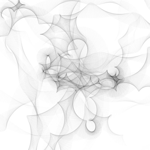
Here’s a code which uses the idea of a “particle system”, i.e. a system which consists of a number of objects (which may vary with time) interacting among themselves, and with their environment. In this case, I have just used 3 particles which are subject to a centripetal force, and that repulse each other. Once you set up a basic interaction system, you can think about how to represent at each time the data produced by the system: in this case I have choose to draw for each particle a rotating line, whose properties, like its transparency, depend on some other parameters (distance from the center).
The interesting thing about using particle systems to make visual art is that in principle one is dealing with a “parameter space”, which doesn’t need to be mapped via the intuition which it was built in the first place with: in other words, there’s no need to represent the objects as actual particles (with positions, velocity, etc.), but one can consider the system as a machine that produces data, to be then represented in the way one artistically feels like. The advantage of using a particle system is that all these data will evolve according to some dynamical evolution which is (in general) not totally random, giving rise to patterns in the final artistic outcome.
int d=3;
Agent[] point=new Agent[d];
void setup(){
randomSeed(90);
size(500,500);
background(255);
for (int i=0;i<d;i++)
{
point[i]= new Agent(random(10,width),random(10,height),random(-1.5,1.5),random(-1.5,1.5));
};
};
void draw(){
for (int i=0;i<d;i++)
{
point[i].resetrep();
for (int j=0;j<d;j++)
{
if (i!=j) point[i].interact(point[j]);
};
};
for (int i=0;i<d;i++)
{
point[i].applyForce();
point[i].move();
point[i].paint();
};
};
class Agent{
PVector loc;
PVector vel;
PVector rep;
float alpha;
int tran;
float l;
float mag=0;
Agent(float _locx,float _locy, float _velx,float _vely){
loc=new PVector(_locx,_locy);
vel=new PVector(_velx,_vely);
rep=new PVector(0,0);
alpha=0;
tran=10;
l=random(20,50);
};
void resetrep(){
rep.x=0;
rep.y=0;
}
void interact(Agent other){
PVector reps=PVector.sub(loc,other.loc);
float m=reps.mag();
reps.normalize();
reps.mult(3/(m+0.0001));
rep.add(reps);
};
void applyForce(){
PVector force=new PVector(random(-0.02,0.02),random(-0.02,0.02));
force.limit(1);
PVector radial=new PVector(-loc.x+width/2,-loc.y+height/2);
mag=-radial.mag();
radial.normalize();
radial.mult(0.022);
force.add(radial);
force.add(rep);
vel.add(force);
vel.limit(6);
};
void move(){
loc.add(vel);
alpha+=2;
};
void paint(){
stroke(int(mag/10),int(mag/10),int(mag/10),int(abs(sin(radians(alpha)*0.1))*10));
pushMatrix();
translate(loc.x,loc.y);
rotate(radians(alpha));
line(-20,0,-20+mag/10+l*(1+abs(sin(radians(alpha)*0.1))),0);
popMatrix();
};
};
Here’s a screenshot of the animation after a few seconds.
27:
The last few days for me have been all about Cellular Automata, due mostly to a long term obsession of mine: complex behaviours of systems at large scale which do not require hierarchy or centralized organization to exist, but “emerge” from local behaviours of the system’s constituents. (Here‘s a TEdTalk by Steven Strogatz on large scale complexity in birds flocks and also inanimate objects.)
What is then a cellular automaton? You can see it as a conceptual building block: it’s an entity capable of being in a given (finite) number of states, and of interacting with its close “neighbours” according to certain very simple rules. The result of the interaction will in general cause a change in the state of the given automaton, and consequently an (discrete time) evolution of the system. The neighbours, once defined, don’t change during the evolution of the system, so, in other words, a cellular automaton is not capable of moving, but it is fixed to a grid, the most common being 1 and 2 dimensional. Moreover, the grid is actually positioned on a circle or torus, so to avoid having to impose boundary conditions, i.e. a modification of the rules for the automata living on the edge of the grid.
Some systems of rules, like Conway’s Game Of Life, which is the one I have used in the code below, and probably the most famous one, exhibit some incredibly interesting global behaviours and patterns.
The code below tries to use Cellular Automata for artistic purposes: some of the parameters of the automaton, as for instance its state, the number of “alive” neighbours, and the number of frames it has been alive, have been used to draw geometric shapes (squares, in this case) of different dimensions, colors,etc. .
Notice that the set of rules is slightly perturbed, so, given an initial state, its evolution is not completely deterministic.
int dim;
Cell[][] cells;
int cellsize=20;
int r=0;
int acc=0;
void setup(){
size(600,600);
background(0);
dim=floor(width/(cellsize/2));
cells=new Cell[dim][dim];
for (int i=0;i<dim;i++)
{
for (int j=0;j<dim;j++)
{
if(random(0,1)<0.7) {r=0;} else {r=1;};
cells[i][j]=new Cell(cellsize/2+i*cellsize/2,cellsize/2+j*cellsize/2,r);
};
};
for (int i=0;i<dim;i++)
{
for (int j=0;j<dim;j++)
{
cells[i][j].paint();
};
};
};
void draw(){
background(0);
nextstateCalc();
for (int i=0;i<dim;i++)
{
for (int j=0;j<dim;j++)
cells[i][j].paint();
};
perturb();
};
;
void nextstateCalc(){
for (int i=0;i<dim;i++)
{
for (int j=0;j<dim;j++)
{
int liveCount=0;
liveCount=cells[(i+dim) % dim][(j+1+dim) % dim].state+cells[(i+1+dim) % dim][(j+1+dim) % dim].state+cells[(i+1+dim) % dim][(j+dim) % dim].state+cells[(i+1+dim) % dim][(j-1+dim) % dim].state+
cells[(i+dim) % dim][(j-1+dim) % dim].state+cells[(i-1+dim) % dim][(j-1+dim) % dim].state+cells[(i-1+dim) % dim][(j+dim) % dim].state+cells[(i-1+dim) % dim][(j+1+dim) % dim].state;
if (cells[i][j].state==1){
cells[i][j].frameAlive++;
if (liveCount == 2 || liveCount == 3) {
cells[i][j].nextstate=1;
}
else {
cells[i][j].nextstate=0;
}
};
if (cells[i][j].state==0){
cells[i][j].frameAlive=0;
if (liveCount == 3) {
cells[i][j].nextstate=1;
};
cells[i][j].neigh=liveCount;
};
};
};
};
void perturb(){
if (random(0,1)<0.1+acc){
int a=int(random(0,dim));
int b=int(random(0,dim));
cells[a][b].state=0;
};
if (acc<=0.9) {
acc+=0.01;
}
else {
acc=0;
}
};
/* Define the cellular automaton class
*/
class Cell{
float x;
float y;
int state;
int nextstate;
int neigh=1;
int frameAlive=0;
Cell (float _x,float _y,int _alive){
x=_x;
y=_y;
state=_alive;
nextstate=_alive;
};
void paint(){
state=nextstate;
noStroke();
fill(150*(neigh),160*(neigh),110*(neigh),4*state);
pushMatrix();
translate(x,y);
rotate(radians(neigh-frameAlive));
rectMode(CENTER);
rect(0,0,3*(1+neigh*(frameAlive % 100)),3*(1+neigh*(frameAlive % 100)));
popMatrix();
};
};
Since the code needs to perform quite a certain load of computations, I have done a render of it, rather than having it running in real time. The music is not strictly speaking related to the animation, but I was inspired by the video to play some piano. 😉
Finally, the use of Cellular Automata was inspired by the reading of Matt Pearson’s very nice Generative Art: A Practical Guide (see also Daniel Shiffmann’s The Nature of Code). I will come back to this topic in a following post, talking about boids and autonomous agents, a somehow related concept. Also, I would like to apply Cellular Automata techniques to sound: I have some ideas, so stay tuned! 😉
02:
Here’s a code in Processing that explores a simple databending technique for images. You can read about Glitch Art , and then start endelessy debate with your friends if this is art or not.
Also, here you can find some interesting series of videos exploring a bit also the philosophy behind databending, glitching and malfunctions as a form of awareness of the technology we are sorrounded by. (A simple example would be how the spelling mistakes in a chat messaging system make you indeed aware of the chat medium itself).
Here’s the code
PImage img;
int width=600;
int height=600;
int x1;
int y1;
int x2;
int y2;
int sx=10;
int sy=100;
int iter=100;
void setup(){
size(width,height);
img=loadImage("rain.jpg");
image(img,0,0);
for (int h=0;h<iter;h++)
{
sx=int(random(5,30));
sy=int(random(50,130));
loadPixels();
x1=int(random(0,width-sx-1));
y1=int(random(0,height-sy-1));
x2=int(random(0,width-sx-1));
y2=int(random(0,height-sy-1));
for (int i=0; i<sx ;i++)
{
for (int j=0; j<sy;j++)
{
color temp=pixels[(x1+i)*width + (y1+j)];
pixels[(x2+i)*width + (y2+j)]=pixels[(x1+int(random(0,i)))*width+(y1+int(random(0,j)))];
pixels[(x1+i)*width + (y1+j)]=temp;
}}
updatePixels();
}
};
The idea is very simple: we “swap” pixel strips of random width and height from the starting image, starting from two random points, and add some jitter to it.
We then iterate the process starting from the last modified image: the parameter iter controls the number of iterations.
Starting from this image (it’s a small piece from an image taken from the web)

I have got this

Of course, you can do a lot more interesting things by accessing directly to the pixels of an image: you can rotate areas, alter colors, etc..
And in particular, you can make animations in Processing using the same principle.
I’ll try to explores this more in future posts, trying maybe also to clear my mind about deconstructivism in art and communications…
01:
Here’s a little code in Processing exploring periodic motion. The single balls have been assigned an angular velocity consisting of “even harmonics”, while the amplitude of the single oscillation is constant up to some tiny random factor, to make the whole animation look more “natural”.
int p=50;
float[] y= new float[p];
float[] r= new float[p+1];
float[] omega= new float[p+1];
float[] amp= new float[p+1];
float t=0;
float s=0;
float b=0;
void setup() {
for (int i=0;i<y.length;i++){
y[i]=i;
};
omega[0]=0;
for (int i=1;i<omega.length;i++){
omega[i]=i*2;
amp[i]=20+random(-1.0,1.0);
};
size(400, 400);
background(255);
}
void draw() {
background(255);
for (int i=0;i<r.length;i++){
r[i]=amp[i]*sin(omega[i]*t/2);
};
for (int i=0;i<y.length;i++){
stroke(50);
strokeWeight(3);
line(width/2+r[i],y[i]*600/p,width/2+r[i+1],y[i]*600/p+600/p);
fill(int(abs(map(sin(i*t/2),-1,1,-255,255))));
strokeWeight(1);
ellipse(width/2+r[i],y[i]*600/p,10,10);
} ;
t +=0.008;
b++;
};
Click below to start/stop the animation.