22:
This post is inspired by some of the stuff Daniel Shiffman has on his YouTube channel.
The idea is based on the use of meshes and textures. So, what’s a mesh and what’s a texture?
A mesh is a collection of vertices, edges and faces that are used in 3D computer graphics to model surfaces or solid objects. If you are familiar with the mathematical notion of a triangulation, you are more or less in business. Even though the faces are not necessarily triangles in general, the analogy works quite well. In Processing there is a nice and quick way to generate a triangular mesh, and it’s via beginShape()/endShape(), which is what I have used in the code below. One starts with a grid (check out some earlier posts for rants about grids), and from the collection of points of the grid Processing will then build a triangular mesh*. This is achieved via the TRIANGLE_STRIP mode: we only need to specify the vertices (though in a precise order), and they will be connected via triangular shapes. Very cool. Ok, we have a tons of little triangles which assemble in a huge square: what do we do with this? Here comes the notion of a texture map. The idea is very simple: we have an image, and we want to “glue” it to a face of the mesh. Once it is glued to such a face, the image will follow the face: for instance, if we rotate such a face, the image which is stuck to that face rotates as well! Now, you should know that mapping textures on a complicated surface is kind of an art, but in our case it is pretty easy, since the surface is just a flat square. To achieve this gluing, we have to define some anchor points in the image. In other words, we have to give information about how points in the original image are associated to vertices in the mesh. The double loop in the code below does exactly this: the last two parameters in the vertex() function specify indeed the gluing.
If we had halted our imagination here, we would end up with something very static: an image attached to a square. Meh. Here comes the simple, but interesting idea. Since we are in 3D geometry, we can modify the z-coordinate of the vertex at point (x,y) with a function of the plane. In this case, the function used is Perlin noise. If we rotate our system of coordinates with respect to the x-axis, you start seeing little mountains appear. Nice! Still, though, there is no movement in place. To achieve such a movement effect, we can increment the y coordinate slightly at each frame, so that the new z-coordinate at point (x, y) will be the value of the z-coordinate at a previous point in the grid, achieving the moving effect. In the code, I’ve furthermore decided to control the offset of the z-coordinate with a variable r whose minimum value is 0, and gets triggered randomly. Notice that I’ve also allowed some “release” time for r, so to achieve some smoothness. In this way you obtain a nice beating feeling. Instead of doing it randomly, what happens if you trigger r via a beat detector listening to some music (using the Sound or Minim library, say)? Yep, you get a nice music visualizer. 
Last couple of things I added is to “move along the image”, and using tint() instead of clearing the screen. The first one is achieved via the variable speed: basically, at each new frame, we don’t glue the image to the mesh in the exact same way, but we translate it a bit in the y-direction.
Oh, I’ve also used more than one image, to get a change in the color palette.
Here’s the code
int w = 1900;
int h = 800;
int cols;
int rows;
int scl = 30;
PImage[] img = new PImage[3];
PImage buff;
float speed = 0.01;
int speed2 = 0;
float r = 0;
void setup() {
size(1200, 720, P3D);
background(0);
//Load the images we are using as textures;
img[0] = loadImage("path_to_image1");
img[1] = loadImage("path_to_image2");
img[2] = loadImage("path_to_image3");
for (int i = 0; i < img.length; i++) {
img[i].resize(1900, 2000);
img[i].filter(BLUR, 0.6);
}
buff =img[0];
noStroke();
cols = w / scl;
rows = h / scl;
}
void draw() {
//Triggers a "beat";
if ( (random(0.0, 1.0) < 0.05) & (r < 0.1) ) {
r = 8.0;
}
//This allows for some release time;
if (r > 0.01) {
r *= 0.95;
}
//From time to time, choose another texture image;
if (random(0.0, 1.0) < 0.008) {
int i = int(random(0, 3));
buff = img[i];
}
float yoff = speed;
speed -= 0.03;
if (frameCount%2 == 0) {
speed2 += 1;
}
speed2 = speed2 % 60;
translate(width/2, height/8);
rotateX(PI/3);
translate(-w/2 + sin(frameCount * 0.003)* 20, -h/2, -450); //The sin function allows for some left/right shift
//Building the mesh
for (int y = 0; y < rows; y++) {
beginShape(TRIANGLE_STRIP);
tint(255, 14);
texture(buff); //Using the chosen image as a texture;
float xoff = 0;
for (int x = 0; x < cols + 1; x++) {
vertex(x * scl, y * scl, map(noise(xoff, yoff), 0, 1.0, -60, 60) * (r + 2.9), x * scl, (y + speed2) % 2000 * scl);
vertex(x * scl, (y + 1) * scl, map(noise(xoff, yoff + 0.1), 0, 1.0, -60, 60) * (r + 2.9), x * scl, ((y + 1 + speed2) % 2000) * scl);
xoff += 0.1;
}
endShape();
yoff += 0.1;
}
}
Here’s it how it looks like
Very floaty and cloud-like, no? 😉
Exercise 1: instead of loading images, use the frames of a video as textures.
Exercise 2: instead of controlling the z-coordinate of a point (x,y) via a Perlin noise function, use the brightness at (x,y) of the texture image obtained in Exercise 1.
Exercise 3: Enjoy.
*One should really think of a mesh as an object which stores information about vertices, edges, etc., while we are here concerned only with displaying a deformed grid.
03:
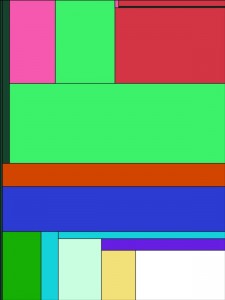
As I mentioned more than once in this blog, one shouldn’t abuse object oriented programming. There is still a lot of beautiful art generated with a few lines of code. I hope the following Processing sketch, inspired by the geometric minimalism of Piet Mondrian, falls in this category
color[] cols;
int num = 5;
void setup() {
size(600, 800);
background(0);
cols = new color[num];
for (int i = 0; i < num; i++) {
cols[i] = color(int(random(0, 255)), int(random(0, 255)), int(random(0, 255)));
}
strokeWeight(1.5);
for (int i = 0; i < 10; i++) {
// rotate(i * 0.1 * 2 * PI);
Mondrian(0, width, height);
}
}
void draw() {
}
void mousePressed() {
fill(255, 255);
rect(0, 0, width, height);
for (int i = 0; i < 10; i++) {
for (int j = 0; j < num; j++) {
cols[j] = color(int(random(0, 255)), int(random(0, 255)), int(random(0, 255)));
}
// rotate(i * 0.1 * 2 * PI);
Mondrian(0, width, height);
}
}
void Mondrian(float x, float len1, float len2) {
if (len1 > 20 & len2 > 20) {
pushMatrix();
translate(x, 0);
color c1 = cols[int(random(0, cols.length))];
if (random(0.0, 1.0) < 0.5) {
float x_new = random(0, len1 * 0.5);
fill(c1, 255);
rect(0, 0, x_new, len2);
Mondrian(x_new, len1 - x_new, len2);
} else {
float len_new = random(0, len2);
fill(c1, 255);
rect(0, 0, len1, len_new);
Mondrian(0, len1, len_new);
}
popMatrix();
}
}
It is essentially based on recursion, and exploits again the idea of a grid, even if in a conceptually different way from the latest post.
If you run the code, you should get something like this
I suggest you uncomment the line which contains the rotate call.
Also, here’s an exercise: modify the function Mondrian() in such a way that the same color is never chosen in successive iteration.
Remark: In his neoplastic paintings, Mondrian used mostly primary colors and white, with white being usually predominant. Moreover, he used thicker lines. Try to modify the code above to achieve the same effect.
07:
I have been working recently on a small audio-visual installation based essentially on grid manipulations, inspired by the art of the amazing Casey Reas.
Grids are some of the first interesting repetitive structures one learns to build. For instance, a one parameter function which displays a regular grid of rectangles maximising the surface of the screen used might look like this
void grid(int n){
float stepx = width/n;
float stepy = height/n;
for (int x = 0; x < width; x+=stepx){
for (int y = 0; y < height; y+=stepy){
rectMode(CENTER);
noStroke();
fill(255);
rect(x + stepx/2.0, y + stepy/2.0, 20, 20);
}
}
}
It will produce a grid of equally spaced white rectangles (so, better set the background to black before in your code). This is all fun and cosy for a couple of milliseconds, but if you are like me, you will look immediately for possibilities of explorations, and honestly the bit of code above doesn’t offer much. Let’s be precise: it *can* offer a lot of ways of tweaking, but they become cumbersome very very quickly. Also, I like to write codes which are conceptually structural and modular, and which allow to separate more clearly the “data holding” part from its representation. I find that this helps a lot the sense of surprise I get from playing with my newly created tool/toy. For instance, all that white is boring: how about we assign a different color to each rectangle? Not randomly though, which would be very cheap. Let’s use an image as a palette, and have each rectangle carry the color of the image pixel at the center of the rectangle. This can be attained by introducing the following line
fill(img.pixels[x + y * width]);
where img is the PImage variable holding your image (which I assume you have resized to the screen width and height, unless you have a fetish for ArrayOutOfBound messages ). Nice. But I guess you still can’t see my point, of course. Okay, let’s do the same but with a video. Now the image is changing at each frame, so the function grid() must be called in the animation loop, i.e. inside draw(). Here you can see my point: by proceding in this way, you are doing a certain amount of redundant computations. Indeed, the only thing that you would like to modify in this case is how each node of the grid is represented, and *not* the grid structure itself. So, it helps then to think of a grid as a data holder for the positions of its nodes, which, once we require some extra properties, are directly determined by a single integer n, the number of nodes per row and column. What we draw on the screen is then a representation of this bunch of information. Anytime you have something that behaves like a collection of data, object oriented programming (OOP) is not far from sight. Building objects (or rather classes) is kind of an art: extracting the relevant properties we want in our objects so that further manipulation becomes reactive and enjoyable is not an easy task. This to say that the are some basic rules in object oriented programming, but for artistic reason we can (and should) ignore many standard design patterns, and look at each case separately. Since I like thinking in terms of objects when programming, I feel the following warning is due: do *not* overuse OOP! There are fantastic pieces of algorithmic/generative art which do not use objects at all. The point is that you might run the risk to decompose the problem in its atomic parts, which has a certain intellectual appeal, no doubt, but then get lost when it comes to exploration and tweaking. So, case by case, see what works best, and, most importantly, what puts you in that spot where you can still get surprised. This said, let’s move on.
So, we can model a grid with the following Grid class
class Grid {
int n;
float[] posx;
float[] posy;
float offsetx;
float offsety;
Shape[] shapes = {};
Grid(int _n){
n = _n;
int stepx = width/n;
int stepy = height/n;
offsetx = stepx/2.0;
offsety = stepy/2.0;
posx = new float[n];
posy = new float[n];
for (int i = 0; i < n; i++){
posx[i] = i * stepx;
posy[i] = i * stepy;
}
for (int i = 0; i < n; i++){
for (int j = 0; j < n; j++){
shapes = (Shape[]) append(shapes,new Shape(posx[i], posy[j]));
}
}
}
Grid(int _n, float _offsetx, float _offsety){
n = _n;
int stepx = width/n;
int stepy = height/n;
offsetx = _offsetx;
offsety = _offsety;
posx = new float[n];
posy = new float[n];
for (int i = 0; i < n; i++){
posx[i] = i * stepx;
posy[i] = i * stepy;
}
for (int i = 0; i < n; i++){
for (int j = 0; j < n; j++){
shapes = (Shape[]) append(shapes,new Shape(posx[i], posy[j]));
}
}
}
Grid(int _n, float len, float _offsetx, float _offsety){
n = _n;
int stepx = int(len/n);
int stepy = int(len/n);
offsetx = _offsetx;
offsety = stepy;
posx = new float[n];
posy = new float[n];
for (int i = 0; i < n; i++){
posx[i] = i * stepx;
posy[i] = i * stepy;
}
for (int i = 0; i < n; i++){
for (int j = 0; j < n; j++){
shapes = (Shape[]) append(shapes,new Shape(posx[i], posy[j]));
}
}
}
void display(){
pushMatrix();
translate(offsetx, offsety);
for (int i = 0; i < shapes.length; i++){
shapes[i].display(20);
}
popMatrix();
}
void display(PImage _img){
_img.loadPixels();
pushMatrix();
translate(offsetx, offsety);
for (int i = 0; i < shapes.length; i++){
shapes[i].setColor(_img.pixels[int(shapes[i].x) + int(shapes[i].y) * _img.width]);
shapes[i].display(20);
}
popMatrix();
}
}
So, you can see that I have heavily used that you can overload constructors and methods, so to give some default behaviours when we don’t want to bother passing a lot of parameters. An instance of Grid will also carry an array of Shape objects: this is the “representational” informations of our grid. Here’s how the Shape class looks like:
class Shape {
float x, y;
color c;
Shape(float _x, float _y){
x = _x;
y = _y;
c = color(255, 255, 255);
}
Shape(float _x, float _y, color _c){
x = _x;
y = _y;
c = _c;
}
void display(float w){
rectMode(CENTER);
noStroke();
fill(c, 255);
rect(x, y, w , w);
rectMode(CORNER);
}
void setColor(color _c){
c = _c;
}
}
If you don’t specify any color, the rectangle will be white.
So, now the previous function grid() is subsumed in the following lines of code
Grid grid = new Grid(20);
grid.display(img);
Apart from the elegance of it, that as I mentioned before should not be the only criterion of judgement, the code now is amenable to vast explorations. For instance, by modifying the display() method of the Shape class we can completely change the appearance of our grid, even so much that it doesn’t look like a grid anymore! Moreover, we don’t have all those redundant computations to be made.
One thing that comes to mind when you have a class is that you can produce many objects from that class with slightly different properties. In this case I have decided to use this expedient in order to explore “fractalization”, which is another (made up?) word for “apply recursion carefully”. Add the following function to your code
void fractalize(int n){
if (n > 1){
grid = new Grid(n, x, y);
grid.display();
x+= grid.offsetx;
y+= grid.offsety;
fractalize(n - 1);
}
}
To make the most of it, you might want to lower the alpha of the filling for the rectangles. Actually, as I mentioned before, we can start exploring the code and the questions it naturally suggests, like: “why restrict ourselves to rectangles?” Or “why even filling them?” “Can I add some stochastic noise here and there to make everything not so hearthless and rigid?” “What is the meaning of life?”
When you start raising these questions, a vast playground (or/and a deep existential pit) opens up.
Believe it or not, after very few adjustments to the Shape class here’s what I got
which I find having an interesting balance between structure and randomness. A nice surprise!
26:
What is and what isn’t generative art is a long standing debate, in which I do not want to enter here. Just to put things in context, though, I’ll share some words about it. For some people, a piece of art is generative if it is the product of some sort of system which, once set in motion, is left to itself, with no further interaction. These systems are also called autonomous. Though generative art is usually associated to algorithmic art, i.e. art generated by some computer algorithm, autonomous systems can be found in biology, chemistry, mechanics, etc. Personally, I find the constraint on the autonomy of the system a bit too tight. While I do think that autonomous systems produce fascinating pieces of art, hence showing the beauty of complexity and emergency, I’m also very much interested in the dichotomy creator/tool, which in this case manifests itself as a shadow of the interaction between human and machine. I’m thinking about art which is computer assisted, more specifically which arises from the interaction of some sort of (algorithmic) system with the creator/spectator. This interaction poses interesting questions. We can indeed consider the total generative system as the combination autonomous system + spectator. This would be an autonomous system itself, if not for one little detail: the spectator is aware (whatever that means) that he’s a tool of a machine which is producing a piece of art. A more concrete example would be the following. Consider a live art installation in which the movements of spectators are used to control some given parameters of a system, which is then used to draw on a big screen, or produce sounds. There is going to be a huge conceptual difference if the spectators are aware of the tracking of their movements or not. In the second case, we are in the presence of something which looks like an autonomous system, while in the first case the spectators could use their awareness to drive the artistic outcome. The topic is incredibly fascinating and worth thinking about: these few words were only meant as a support to the fact that I would consider as generative art* the piece that you are going to see in the following.
Since discussions surrounding art are not notoriously controversial enough, I’ll move to noise and randomness (yeeeih!). Let’s start with saying: you can’t generate random numbers with a computer. Behind any random number produced with a programming language, there is an algorithm: in general it is a very complicated one and takes as parameter physical parameters of your machine (say, the speed of the CPU at the moment you request a random number), but it is still an algorithm. It is just so complex that we (as humans) can’t see any logical pattern behind it. I already feel the objection coming: “Well, what is randomness anyway? Is there anything truly random?”. I’m going to skip this objection quickly, pointing here instead. Enjoy! 😉
Processing offers two functions to treat randomness and noise: one is random(), and the other is noise(). Actually, noise() is a function that reproduces Perlin noise, a type of gradient noise which is extremely useful to reproduce organic textures.
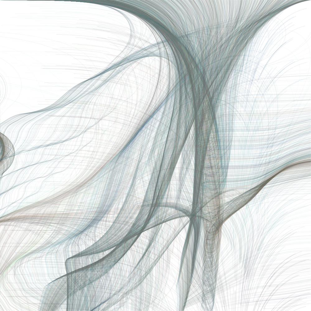
Though Perlin noise is great, no doubt about that, and since randomness for a machine is just a function which looks unpredictable, why not make one’s own noise? After all, one of the point of generative art is that it allows to build tools which can be played with and explored. The function customNoise() in the code below does exactly that: it is a function from -1 to 1 which behaves in an erratic enough way to be a good substitute for noise(). You have now got your very own noise function, well done! The question is: what are we going to do with that? That’s where the second noun in the title of this post enters the stage. Every time you have a nice function in two variables, you can build out of it a vector field. “What’s that?”, you might say. You can think of it as an assignment of a little arrow to each point of the screen, with the angle (in this case) respect to the x-axis determined by our noise function. Once we have such a little arrow, we can use it to tell a particle which is at a given position on the screen where to go next. You can imagine the vector field as being associated to a fluid which at each point moves exactly with velocity given by the value of the vector field. If you then drop tiny particles in the fluid, they will start moving along curves, which are called the flow curves of the vector field. Moreover, they will start accumulate along specific flow curves: I leave you to investigate why it is that. 😉
So, the following Processing code brings home all these ideas, plus a last one, which has to do with the beginning of this post. You will notice that the function customNoise() has a mouseX inside, and there’s a mouseY controlling the variable depth. This means that the function interacts with the mouse movement, and hence the output of the code can be driven by the user. In particular, the piece you get stays comfortably in that gray area between generative and nongenerative art, one of those interesting arguments you can entertain your friends with at the next vernissage or pub quiz you go. 😉
Here’s the code:
float[] x;
float[] y;
color[] col;
float s = 0.001;
float depth = 0.5;
PImage img;
void setup() {
size(1000, 1000);
background(0);
int n = 1000;
x = new float[n];
y = new float[n];
col = new color[n];
img = loadImage(pathtoimage/image);
img.resize(width, height);
img.loadPixels();
for (int i = 0; i < x.length; i++) {
x[i]= random(0, width);
y[i]= random(0, height);
int loc = int(x[i]) + int(y[i])*width;
col[i] = img.pixels[loc];
}
}
void draw() {
noStroke();
depth = map(mouseY, 0, height, 0.5, 1.5);
//fill(255, 4); //Uncomment if you don't want to use an image;
for (int i = 0; i < x.length; i++) {
float alpha = customNoise(x[i] * s, y[i] * s)*2*PI;
x[i]+= depth * cos(alpha); // + random(-0.4, 0.4);
y[i]+= depth * sin(alpha); // + random(-0.4, 0.4);
if (y[i] > height) {
y[i] = 0;
x[i] = random(0, width);
}
x[i]= x[i]%width;
fill(col[i], 4); //Comment if you don't want to use an image;
ellipse(x[i], y[i], 2, 2);
}
}
float customNoise(float x, float y) {
return pow(sin(0.9*x + noise(x, y)*map(mouseX, 0, width, 0, 5)*y), 3);
}
You will get something like this
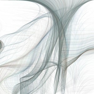
Notice that the first piece is obtained by commenting/uncommenting some few lines.
Finally, there is one last question you might ask, and it is the following:”How did you come up with those peculiar numbers for the parameters in the code?”. Well, the answer is: by a certain amount of trial and error. As I mentioned more than once, making art with code allows for a great degree of exploration: tweaking a parameter here and changing a line there can give you very different and unexpected results. That what you get at the end is artistically appealing or not, well, nobody else can tell but you. These highly subjective decisions are what transforms a bunch of programming lines into something meaningful and beautiful. So, go on tweaking and looking for something you find interesting and worth sharing, then!
*If you are post-modernly thinking “Who cares if it’s called generative or not?”, you definitely have all my sympathy.
21:
Digital poetry is that part of literature which is concerned with poetic forms of expression which are mainly computer aided. I am using the term in a strong sense here, i.e. I am thinking about generative poetry, hypertext poetry, and for this occasion in particular digital visual poetry. In general, the relation between the (graphical) sign used to represent a word and its actual meaning in a poetic text is a very interesting (and crucial) one. Indeed, the way words are represented can be an integral part of the aesthetic value of a piece of literary text, poetry in this case. Just think about the beautiful art of Chinese calligraphy, for example. It is then not surprising that poetry, as many forms of digital art, can be glitched* too. I have written about glitch art already, and we can use a couple of ideas and methodology from there. One way to glitch a piece of poetry would be to introduce orthographic anomalies/errors in the text to get for instance something like**
“SnOww i% my s!hoooe
AbanNdo;^^ed
Sparr#w^s nset”
At this stage we are working mainly with the signifier, but in a way which doesn’t take into account the actual spatial representation of the text itself. (Yes, the text is actually represented already, I’m being a bit sloppy here.)
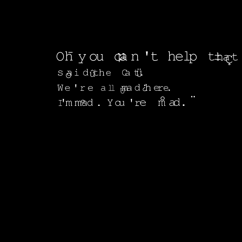
More in the direction of digital visual poetry, we can work with properties of the visualized text: the position of the actual characters involved, for instance. The graphical atoms will be then the characters forming the words in the text, in this case, and we introduce perturbations to their positions in space, and some other visual artifacts. To achieve this, we can regard the various lines of text, which are of type String, as array of characters, and display them. We have then to take care of the length in pixels of each character with the function textWidth(), in order to be able to display the various lines of text.
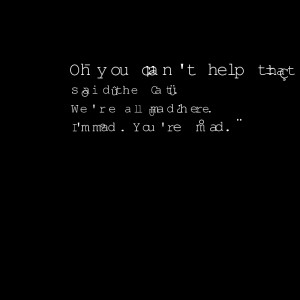
Here’s how a simple Processing code inspired by these ideas would look like:
PFont font;
String[] text = {"Oh you can't help that,", "said the Cat.", "We're all mad here.", "I'm mad. You're mad." };
int size = 48;
int index = 0;
void setup(){
size(800, 800);
background(0);
textAlign(CENTER);
font = loadFont("TlwgTypewriter-48.vlw"); //You can create fonts with Tools/Create Font in Processing
textFont(font, size);
for (int i = 0; i < text.length; i++){
float posx = 200;
float posy = 200 + i * 50;
for (int j = 0; j < text[i].length(); j++){
textSize(size);
text(text[i].charAt(j), posx, posy);
posx = posx + textWidth(text[i].charAt(j)) +random(-10, 10);
if (random(0.0, 1.0) < 0.3){
size = size + int(random(-10, 10));
glitch(posx, posy);
}
}
}
}
void draw(){
}
void glitch(float x, float y){
char c = char(int(random(130, 255)));
text(c, x + random(-10, 10), y + random(-10, 10));
}
You would get something like this
I have been lazy, and introduced the array of strings directly in the code: an easy (but instructive) variation would be to load a piece of text from a .txt file, and parse it to obtain the individual lines.
Finally, we could work at a third layer of graphic “deepness”: we could consider the whole text as an image, and use the ideas in the previous post to glitch it. This is left to you as an interesting exercise.
Most importantly: never contradict the Cheshire Cat, mind you. 😉
*I avoid using the term “hacked”, since nowadays it is practically and culturally meaningless. Someone suggested “hijacked”, which I prefer.
** Thanks to Kerouac for the raw material to esperiment with.
17:
This code is a nice playground for some advanced aspects of Object Oriented Programming (OOP): it is simple enough to be interesting, and show the power and elegance of a more abstract approach to programming. What does the code do? It generates a number of bouncing particles which disappear when colliding with each other. Pretty simple. Now, in general, when you have to test a condition for an object against the totality of objects present, you may run soon in annoying cycles which can obscure the code itself, making it less readable, and which would be best avoided. To do this, I need to introduce one easy, but extremely important observation on how function in Processing (and Java, and many other languages) work: “Objects to a function are passed by reference“. Remember this, write it somewhere, do whatever but don’t forget it. “Oookay”, you say, “but, what does “passed by reference” even mean? What’s a “reference”?”. In OOP, objects are instantiated as initialized references, which means the following: suppose we have a class Ball (with empty constructor), and the following piece of code
In plain English, the code above says: create a label p which labels an object of type Ball, then create an object of type Ball, and attach to it the label p. In other words, p is *not* the object*, but it is just a label “referencing” the actual Ball object. Indeed, if we add the following piece of code
we are asking to create a new label q, referencing to the same object p is referencing. Now, as soon as we modify the actual object which is referenced, these modifications will reflect on the behaviour of p and q. For instance, suppose that the class Ball has a field a, of type integer, which is initialized to 10. Then the following code
println(q.a);
p.a = 15;
println(q.a);
will return 10, and then 15. In other words, changing p has changed *also* q, and the reason is that we are really not changing p, but rather the object p references to. A bit confusing, right? Neverthless I bet you have seen this behaviour before, if you have ever used (and who hasn’t) arrays.
Indeed, this piece of code would give the same results;
int[] p = new int[10];
int[] q;
q = p;
q[0] = 10;
p[0] = 15;
println(q[0]);
Okay, we are ready to talk about “passing by reference”**. Suppose you have a function
void f(Ball b){
do something;
}
and suppose we evaluate it on p, as in f(p). What happens is that b becomes a reference to the object referenced by p (as in b = p). So, if you modify b inside the scope of f, then you are really modifying the referenced object, and hence also p. Of course, the same is true for arrays, so be careful with what you do inside the scope of a function, when arrays are involved.
Supposing this is more or less, clear, the question remains: why caring about this for some stupid balls? Well, this simple observation allows to define something like this
class Ball{
int a;
Ball[] balls;
Ball(int _a, Ball[] _balls){
a = 10;
balls = _balls;
}
}
Wait, what’s going on here? Am I defining a class Ball in which one of its fields is an array of objects of type… Ball?! Like, isn’t there gonna be a nasty recursion type of end of the universe OMG!!
Calm down, nothing’s bad gonna happen. And the reason lies in the simple observations above: objects variable (and arrays) are defined as reference, and they need to be initialized. In the case above, we are asking for a label balls which is a reference to an array of type Ball: at this point we are *not* calling the constructor Ball( ). When it will be called, though, the array balls will reference to the same array referenced by the label (or variable) _balls. Here we are using that objects are passed to functions by reference (the constructor, in this case). Nice, uh?
Notice that, on the other hand, this piece of code
class Ball{
int a;
Ball p;
Ball(int _a){
a = 10;
p = new Ball();
}
}
will give a nasty recursion, since we are indeed calling the constructor inside itself.
Ok, still, what do we do with this?
Here’s the Processing code
int num = 50;
ArrayList<Particle> partls;
void setup(){
size(600, 600);
background(0);
partls = new ArrayList<Particle>();
for (int i = 0; i < num; i++){
partls.add(new Particle(random(0, width), random(0, height), partls));
}
}
void draw(){
ArrayList<Particle> remove = new ArrayList<Particle>();
background(0);
for (Particle par: partls){
par.update();
par.display();
}
for (Particle par: partls){
if (par.collide()) remove.add(par);
}
for (Particle par: remove){
partls.remove(par);
}
}
///Define the class Particle
class Particle{
float x, y, vx, vy, r;
ArrayList<Particle> others;
Particle(float _x, float _y, ArrayList<Particle> _others){
x = _x;
y = _y;
vx = random(-5, 5);
vy = random(-5, 5);
others = _others;
r = 20;
}
void update(){
if ( x <=0 || x >= width) vx = -vx;
if ( y <=0 || y >= height) vy = -vy;
x = (x + vx);
y = (y + vy);
}
void display(){
fill(255, 200);
ellipse(x, y, r, r);
}
boolean collide(){
boolean b = false;
for (Particle p: others){
if (dist(x, y, p.x, p.y) <= r & dist(x, y, p.x, p.y) > 0.0){
b = true;
}
}
return b;
}
}
Let’s look at the Particle class. Among other fields, we have others, an ArrayList of type Particle, which refers to the ArrayList _others passed to the constructor. The variable others is used in the method collide, which tests the distance between the instantiated object and all the particles in the list others, and returns the value true if a collision happens (the condition dist(x, y, p.x, p.y) > 0.0 ensures no self-collision). Also, notice the “enhanced” for loop, which is pretty elegant.
Now, the magic appears in the main code, namely in
partls = new ArrayList();
for (int i = 0; i < num; i++){
partls.add(new Particle(random(0, width), random(0, height), partls));
}
The first line initializes the variable partls as an (empty) ArrayList of type Particle. In the for loop, we add to partls some objects of type Particle by passing to the constructor the required fields: x, y, and others. Since objects are passed by reference to the constructor, this means that, at the end of the for loop, for each object instance of Particle the field others will reference to the same ArrayList referenced by partls, which, by construction, is an ArrayList in which each element is exactly the object Particle created in the for loop. The reference partls gets modified at each iteration of the cycle, and since we are passing it by reference, this modification will reflect also on the variable others. Pretty cool, uh?
This is quite a convenient way to manage collisions. Indeed, in the draw() function we have first the usual (enhanced) for loop which updates, and displays the particles. Then we check for collisions: if the particle collides with any other particle, we add it to a remove list. We need to do this, instead of removing it on the spot, because otherwise only one of the two particles involved in a collision would get removed. Finally, we have another for loop, in order to dispose of the colliding particles.
Everything is pretty elegant and compact, and most importantly, the code is more readable this way!
No video this time, since it’s pretty visually uninteresting.
*Not 100% true, but pretty close.
**There exists also the notion of “passing by value”.
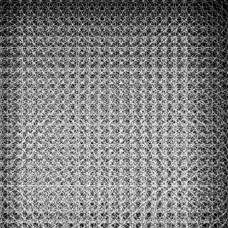
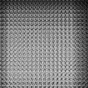
13:
It has been a while since my last update, and in particular since my last Processing code! So, here’s something very simple. Basically, it’s a grid of points connected by lines, which form the edges of polygons. The points move almost periodically: each of them undergoes an oscillatory motion, to which I’ve added a bit of noise, to make things more interesting. The polygons, which during the motion change their shape as the vertices move, are colored. Here comes the nice part: the color of a single polygon is given by taking at its geometric center the color of the pixel of the image obtained by capturing a frame via the webcam. In this way, the colors are “smeared”, but you can still somehow discern the webcam input. Here’s the code.
import processing.video.*;
Capture cam;
int n = 30;
float t = 0;
Point[][] points = new Point[n][n];
void setup(){
size(320, 240);
cam = new Capture(this, 320, 240, 30);
cam.start();
background(0);
/* Setup the grid;
for (int i = 0; i < n; i++)
{
for (int j = 0; j < n; j++)
{
points[i][j] = new Point(i*width/n, j*height/n);
}
}
}
void draw(){
if(cam.available()) {
cam.read();
}
background(0);
for (int i = 0; i < n; i++)
{
for (int j = 0; j < n; j++)
{
points[i][j].move();
points[i][j].display();
}
}
grid(points);
t+= 0.1;
}
void grid(Point[][] gr){
int c_x, c_y;
for (int i = 0 ; i < n; i++){
for (int j = 0; j < n; j++){
if ( j < n -1 && i < n - 1){
stroke(255, 100);
/* Compute the geometric center;
c_x = constrain(int((gr[i][j].pos.x + gr[i][j + 1].pos.x + gr[i + 1][j + 1].pos.x + gr[i + 1][j].pos.x)/4), 0, width);
c_y = constrain(int((gr[i][j].pos.y + gr[i][j + 1].pos.y + gr[i + 1][j + 1].pos.y + gr[i + 1][j].pos.y)/4), 0, height);
/* Create the polygon;
fill(cam.pixels[constrain(c_x + width*c_y, 0, cam.pixels.length - 1)], 250);
beginShape();
vertex(gr[i][j].pos.x, gr[i][j].pos.y);
vertex(gr[i][j + 1].pos.x, gr[i][j + 1].pos.y);
vertex(gr[i + 1][j + 1].pos.x, gr[i + 1][j + 1].pos.y);
vertex(gr[i + 1][j].pos.x, gr[i + 1][j].pos.y);
endShape();
}
}
}
}
/* Define the class Point
class Point{
PVector pos;
float angle;
float depth;
PVector dir;
float phase;
float vel;
Point(float _x, float _y){
pos = new PVector(_x, _y);
angle = random(0.0, 2*PI);
depth = random(0.8, 2.4);
dir = new PVector(cos(angle), sin(angle));
vel = random(0.5, 1.5);
}
void display(){
noStroke();
fill(255, 255);
ellipse(pos.x, pos.y, 4, 4);
}
void move(){
/* Oscillatory motion with noise which depends on the "time" variable t;
pos.x = pos.x + dir.x * cos(vel*t + noise(t*angle)*0.1) * depth;
pos.y = pos.y + dir.y * cos(vel*t + noise(t*angle)*0.1) * depth;
}
}
Warning: Kids, don’t code the way I do! In this case I was particularly lazy: indeed, a more elegant way to do it would have been to create another class, say Grid, and hide there the polygon making, etc. The code would have been more readable and reusable, that way. But as I said, lazyness.
Here’s a little video of what you get
(If it doesn’t work, you can download or stream this )
05:
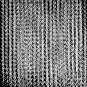
I am not usually excited about the sketches I make in Processing: I mean, I do like them, but I always think they could have come out better, somehow.
This one, instead, I really like, and I’m quite happy about. It is the outcome of playing with an amazing particle systems library for Processing, called toxiclibs.
The whole idea is particularly simple: take a huge number of points, and connect them with springs with a short rest length, so to form a circular shape. Moreover, add an attraction towards the center, and start the animation with the particles far from the center. They’ll start bouncing under elastic forces and the attraction to the center until the circular shape becomes relatively small. The interesting choice here, from the visual perspective, was not to “represent” (or draw) the particles, but rather the springs themselves. One of the important feature of the animation, in this case, is to be able to slowly clean the screen from what has been drawn on it, otherwise you’ll end up with a huge white blob (not that pleasant, is it?). This is accomplished by the function fadescr, which goes pixel by pixel and slowly turns it to the value 0 in all of its colour channels, so basically fading the screen to black: all the >> and << binary operations are there to speed up things, which is crucial in these cases.
Why not using the celebrated "rectangle over the screen with low alpha"? Because it produces "ghosts", or graphic artifacts. See here for a nice description.
I really like the type of textures the animation develops, it gives me the idea of smooth silk, smoke or… flares. 😉
import toxi.physics2d.*;
import toxi.physics2d.behaviors.*;
import toxi.geom.*;
VerletPhysics2D physics;
int N=2000;
VerletParticle2D[] particles=new VerletParticle2D[N];
VerletParticle2D center;
float r=200;
void setup(){
size(600,600);
background(0);
frameRate(30);
physics=new VerletPhysics2D();
center=new VerletParticle2D(new Vec2D(width/2,height/2));
center.lock();
AttractionBehavior behavior = new AttractionBehavior(center, 800, 0.01);
physics.addBehavior(behavior);
beginShape();
noFill();
stroke(255,5);
for (int i=0;i<particles.length;i++){
particles[i]=new VerletParticle2D(new Vec2D(width/2+(r+random(10,30))*cos(radians(i*360/N)),height/2+(r+random(10,30))*sin(radians(i*360/N))));
vertex(particles[i].x,particles[i].y);
}
endShape();
for (int i=0;i<particles.length;i++){
physics.addParticle(particles[i]);
};
for (int i=1;i<particles.length;i++){
VerletSpring2D spring=new VerletSpring2D(particles[i],particles[i-1],10,0.01);
physics.addSpring(spring);
};
VerletSpring2D spring=new VerletSpring2D(particles[0],particles[N-1],20,0.01);
physics.addSpring(spring);
};
void draw(){
physics.update();
beginShape();
noFill();
stroke(255,10);
for (int i=0;i<particles.length;i++){
vertex(particles[i].x,particles[i].y);
}
endShape();
if (frameCount % 3 == 0)
{
fadescr(0,0,0);
};
};
void fadescr(int r, int g, int b) {
int red, green, blue;
loadPixels();
for (int i = 0; i < pixels.length; i++) {
red = (pixels[i] >> 16) & 0x000000ff;
green = (pixels[i] >> 8) & 0x000000ff;
blue = pixels[i] & 0x000000ff;
pixels[i] = (((red+((r-red)>>8)) << 16) | ((green+((g-green)>>8)) << 8) | (blue+((b-blue)>>8)));
}
updatePixels();
}
Here’s a render of the animation
The audio has been generated in SuperCollider, using the following code
s.boot;
~b=Bus.audio(s,2);
File.openDialog("",{|path|
~path=path;
~buff=Buffer.read(s,path);
})
20.do({
~x=~x.add(Buffer.read(s,~path,rrand(0,~buff.numFrames)));
})
(
SynthDef(\playbuff,{arg out=0,in=0,r=1,p=0;
var sig=PlayBuf.ar(1,in,r,loop:1);
var env=EnvGen.kr(Env([0,1,1,0],[0.01,Rand(0.1,1),0.01]),gate:1,doneAction:2);
Out.ar(out,Pan2.ar(sig*env*3,pos:p));
}).add;
SynthDef(\synth,{arg out=0;
var sig=VarSaw.ar(90,0,0.5*LFTri.kr(0.1).range(1,1.2),mul:0.1)+VarSaw.ar(90.5,0,0.5*LFTri.kr(0.2).range(1,1.2),mul:0.1)+VarSaw.ar(90.8,0,0.5*LFTri.kr(0.3).range(1,1.2),mul:0.1);
sig=HPF.ar(sig,200);
sig=FreeVerb.ar(sig);
Out.ar(out,sig!2)
}).add;
SynthDef(\pad,{arg out=0,f=0;
var sig=Array.fill(3,{|n| SinOsc.ar(f*(n+1),0,0.05/(n+1))}).sum;
var env=EnvGen.kr(Env([0,1,1,0],[10,5,10]),gate:1,doneAction:2);
sig=LPF.ar(sig,3000);
Out.ar(~b,sig*env!2)
}).add;
SynthDef(\del,{arg out=0;
var sig=CombC.ar(In.ar(~b,2),0.4,TRand.kr(0.05,0.3,Impulse.kr(0.1)),7);
Out.ar(out,sig);
}).add;
)
y=Synth(\del);
x=Synth(\synth);
t=fork{
inf.do{
Synth(\pad,[\f:[48,52,53,55,57].choose.midicps]);
23.wait;}
};
q=fork{
inf.do{
Synth(\playbuff,[\in:~x[rrand(0,20).asInteger],\r:[-1,1].choose,\p:rrand(-0.5,0.5),\out:[0,~b].wchoose([0.92,0.08])]);
rrand(0.5,3).wait}
}
t.stop;
q.stop;
x.free;
y.free;
s.quit;
28:
In this post I’ll not show you any code, but I want to talk about coding, instead, in particular about “live coding”.
All the various codes you have seen on this blog share a common feature: they are “static”.
I’ll try to explain it better.
When you write a code in a programming language, you may have in mind the following situation: you write down some instructions for the machine to execute, you tell the compiler to compile, and wait for the “result”. By result here I don’t mean simply a numerical or any other output which is “time independent”: I mean more generally (and very vaguely) the process the machine was instructed to perform. For instance, an animation in Processing or a musical composition in SuperCollider is for sure not static by any mean, since it requires the existence of time itself to make sense. Neverthless, the code itself, once the process is happening (at “runtime”), it is static: it is immutable, it cannot be modified. Imagine the compiler like an orchestra director, who instructs the musicians with a score written by a composer: the composer cannot intervene in the middle of the execution, and change the next four measures for the violin and the trombone. Or could he?
Equivalentely, could it be possible to change part of a code while it is running? This would have a great impact on the various artistic situations where coding it is used, because it would allow to “improvise” the rules of the game, the instructions the machine was told to blindly follow.
The answer is yeah, it is possible. And more interestingly, people do it.
According to the Holy Grail of Knowledge
”Live coding (sometimes referred to as ‘on-the-fly programming’, ‘just in time programming’) is a programming practice centred upon the use of improvised interactive programming. Live coding is often used to create sound and image based digital media, and is particularly prevalent in computer music, combining algorithmic composition with improvisation.”
So, why doing live coding? Well, if you are into electronic music, maybe of the dancey type, you can get very soon a “press play” feeling, and maybe look for possibilities to improvise (if you are into improvising, anyways).
It may build that performing tension, experienced by live musicans, for instance, which can produce nice creative effects. This doesn’t mean that everything which is live coded is going to be great, in the same way as it is not true that going to a live concert is going to be a great experience. I’m not a live coder expert, but I can assure you it is quite fun, and gives stronger type of performing feelings than just triggering clips with a MIDI controller.
If you are curious about live coding in SuperCollider, words like ProxySpace, Ndef, Pdef, Tdef, etc. will come useful. Also, the chapter on Just In Time Programming from the SuperCollider Book is a must.
I realize I could go on blabbering for a long time about this, but I’ll instead do something useful, and list some links, which should give you an idea on what’s happening in this field.
I guess you can’t rightly talk about live coding without mentioning TOPLAP.
A nice guest post by Alex Mclean about live coding and music.
Here’s Andrew Sorensen live coding a Disklavier in Impromptu.
Benoit and The Mandelbrots, a live coding band.
Algorave: if the name does suggest you that it’s algorithmic dancey music, then you are correct! Watch Norah Lorway perform in London.
The list could go on, and on, and on…
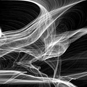
18:
This code came out by playing with particle systems in Processing.
I have talked about particle systems in the post before in the context of generating a still image. In this particle system there is an important and conceptual difference, though: the number of particles is not conserved. Each particle has a life span, after which the particle is removed from the system: this is done by using ArrayList rather than a simple array. In the rendered video below, you will see clearly that particles start to disappear. The disappearing of particles could have been in principle obtained by simply gradually reducing the opacity of a given particle to 0, rather than removing it: in other words, the particle is still there, it’s only invisible. In the particle system I have used, the two approaches make no difference, apart from saving computational resources (which still is a big deal!), since the particles do not interact among each other. If inter particle interactions were present, the situation would be completely different: an invisible particle would still interact with the others, hence it would not be really “dead”.
Believe it or not, to accept the fact that the number of particles in a system might not be conserved required at the beginning of the 20th century a huge paradigm shift in the way physical systems, in particular at the quantum scale, are described, giving a good reason (among others) to develop a new physical framework, called Quantum Field Theory.
import processing.opengl.*;
int N=500*30;
ArrayList<Part> particles= new ArrayList<Part>();
float t=0;
float p=1;
float centx,centy,centz;
float s=0.01;
float alpha=0;
float st=0;
void setup(){
size(500,500,OPENGL);
background(0);
directionalLight(126, 126, 126, 0, 0, -1);
ambientLight(102, 102, 102);
centx=width/2;
centy=height/2;
centz=0;
for (int i=0;i<N;i++){
float r=random(0,500);
float omega=random(0,360);
particles.add(new Part(new PVector(width/2+r*sin(radians(omega)),height/2+r*cos(radians(omega)),0)));
};
for (int i=0;i<particles.size();i++){
Part p=particles.get(i);
p.display();
};
};
void draw(){
if (random(0.0,1.0)<0.01) {
t=0;
st=random(0.002,0.003);
p=random(1.0,1.3);
};
s+=(st-s)*0.01;
background(0);
directionalLight(255, 255, 255, 0, 4, -10);
ambientLight(255, 255, 255);
centx=width/2+400*abs(sin(alpha/200))*sin(radians(alpha));
centz=0;
centy=height/2+400*abs(sin(alpha/200))*cos(radians(alpha));
for (int i=particles.size()-1;i>=0;i--){
Part p=particles.get(i);
p.run();
if (p.isDead()) particles.remove(i);
};
t+=0.01;
alpha+=5;
};
%%%%Define the class Part
class Part{
PVector loc;
PVector vel;
float l;
float lifesp;
Part(PVector _loc){
loc=_loc.get();
vel=new PVector(random(-0.5,0.5),random(-0.5,0.5),0.1*random(-0.1,0.1));
l =random(2.0,5.0);
lifesp=random(255,2000);
};
void applyForce(float t){
PVector f= newPVector(random(-0.1,0.1)*sin(noise(loc.x,loc.y,t/2)),random(-0.1,0.1)*cos(noise(loc.x,loc.y,t/2)),0.01*sin(t/10));
f.mult(0.1*p);
vel.add(f);
PVector rad=PVector.sub(new PVector(centx,centy,centz-50),loc);
rad.mult(s);
rad.mult(0.12*(l/2));
vel.add(rad);
vel.limit(7);
};
void move(){
loc.add(vel);
lifesp-=1;
};
void display(){
noStroke();
fill(255,random(130,220));
pushMatrix();
translate(loc.x,loc.y,loc.z);
ellipse(0,0,l,l);
popMatrix();
};
void run(){
applyForce(t);
move();
display();
};
boolean isDead(){
if (lifesp<0.0){
return true;
} else {
return false;
}
}
};
Here you find a render of the video (which took me quite some time…), which has being aurally decorated with a spacey drone, because… well, I like drones. 😉